NumPy is, just like SciPy, Scikit-Learn, pandas, and similar packages. They are the Python packages that you just can’t miss when you’re learning data science, mainly because this library provides you with an array data structure that holds some benefits over Python lists, such as being more compact, faster access in reading and writing items, being more convenient and more efficient.
This NumPy will focus precisely on this. It will not only show you what NumPy arrays actually are and how you can install Python, but you’ll also learn how to make arrays (even when your data comes from files), how broadcasting works, how you can ask for help, how to manipulate your arrays and how to visualize them.
If you want to know even more about NumPy arrays and the other data structures that you will need in your data science journey, consider taking a look at DataCamp’s Intro to Python for Data Science, which has a chapter on NumPy.
What is a Python Numpy Array?
You already read in the introduction that NumPy arrays are a bit like Python lists, but still very much different at the same time. For those of you who are new to the topic, let’s clarify what it exactly is and what it’s good for.
As the name gives away, a NumPy array is a central data structure of the numpy library. The library’s name is short for “Numeric Python” or “Numerical Python.”
In other words, NumPy is a Python library that is the core library for scientific computing in Python. It contains a collection of tools and techniques that can be used to solve mathematical models of problems in science and engineering.
One of these tools is a high-performance multidimensional array object that is a powerful data structure for the efficient computation of arrays and matrices. To work with these arrays, there’s a vast amount of high-level mathematical functions operate on these matrices and arrays.
But what is an array?
When you look at the print of a couple of arrays, you could see it as a grid that contains values of the same type:
import numpy as np
# Define a 1D array
my_array = np.array([[1, 2, 3, 4],
                     [5, 6, 7, 8]],
                    dtype=np.int64)
# Define a 2D array
my_2d_array = np.array([[1, 2, 3, 4],
                        [5, 6, 7, 8]],
                       dtype=np.int64)
# Define a 3D array
my_3d_array = np.array([[[1, 2, 3, 4],
                         [5, 6, 7, 8]],
                        [[1, 2, 3, 4],
                         [9, 10, 11, 12]]],
                       dtype=np.int64)
# Print the 1D array
print("Printing my_array:")
print(my_array)
# Print the 2D array
print("Printing my_2d_array:")
print(my_2d_array)
# Print the 3D array
print("Printing my_3d_array:")
print(my_3d_array)
You see that, in the example above, the data are integers. The array holds and represents any regular data in a structured way.
However, you should know that, on a structural level, an array is basically nothing but pointers. It’s a combination of a memory address, a data type, a shape, and strides:
- The data pointer indicates the memory address of the first byte in the array.
- The data type or dtype pointer describes the kind of elements that are contained within the array.
- The shape indicates the shape of the array.
- The strides are the number of bytes that should be skipped in memory to go to the next element. If your strides are (10,1), you need to proceed one byte to get to the next column and 10 bytes to locate the next row.
In other words, an array contains information about the raw data, how to locate an element, and how to interpret an element.
Enough of the theory. Let’s check this out ourselves:
You can easily test this by exploring the numpy array attributes:
import numpy as np
my_2d_array = np.array([[1,2,3,4], [5,6,7,8]], dtype=np.int64)

# Print out memory address
print(my_2d_array.data)

# Print out the shape of `my_array`
print(my_2d_array.shape)

# Print out the data type of `my_array`
print(my_2d_array.dtype)

# Print out the stride of `my_array`
print(my_2d_array.strides)
You see that now, you get a lot more information: for example, the data type that is printed out is ‘int64’ or signed 32-bit integer type; This is a lot more detailed! That also means that the array is stored in memory as 64 bytes (as each integer takes up 8 bytes and you have an array of 8 integers). The strides of the array tell us that you have to skip 8 bytes (one value) to move to the next column, but 32 bytes (4 values) to get to the same position in the next row. As such, the strides for the array will be (32,8).
Note that if you set the data type to int32, the strides tuple that you get back will be (16, 4), as you will still need to move one value to the next column and 4 values to get the same position. The only thing that will have changed is the fact that each integer will take up 4 bytes instead of 8
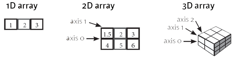
The array that you see above is, as its name already suggested, a 2-dimensional array: you have rows and columns. The rows are indicated as the “axis 0”, while the columns are the “axis 1”. The number of the axis goes up accordingly with the number of the dimensions: in 3-D arrays, of which you have also seen an example in the previous code chunk, you’ll have an additional “axis 2”. Note that these axes are only valid for arrays that have at least 2 dimensions, as there is no point in having this for 1-D arrays;
These axes will come in handy later when you’re manipulating the shape of your NumPy arrays.
How to Install Numpy
Before you can start to try out these NumPy arrays for yourself, you first have to make sure that you have it installed locally (assuming that you’re working on your pc). If you have the Python library already available, go ahead and skip this section :)
If you still need to set up your environment, you must be aware that there are two major ways of installing NumPy on your pc: with the help of Python wheels or the Anaconda Python distribution.
Install With Python Wheels
Make sure firstly that you have Python installed. You can check out our guide on how to install Python if you still need to do this :)
If you’re working on Windows, make sure that you have added Python to the PATH environment variable. Then, don’t forget to install a package manager, such as pip, which will ensure that you’re able to use Python’s open-source libraries.
Note that recent versions of Python 3 come with pip, so double-check if you have it, and if you do, upgrade it before you install NumPy:
pip install pip --upgrade
pip --versionpip install numpy-<version>-<architecture>.whlpip install numpy-1.20.3-cp39-cp39-win_amd64.whlimport numpyInstall With the Anaconda Python Distribution
To get NumPy, you could also download the Anaconda Python distribution. This is easy and will allow you to get started quickly! If you haven’t downloaded it already, go to the official page to get it. Follow the instructions to install, and you're ready to start!
Do you wonder why this might actually be easier?
The good thing about getting this Python distribution is the fact that you don’t need to worry too much about separately installing NumPy or any of the major packages that you’ll be using for your data analyses, such as pandas, scikit-learn, etc.
Because, especially if you’re very new to Python, programming or terminals, it can really come as a relief that Anaconda already includes 100 of the most popular Python, R, and Scala packages for data science. But also for more seasoned data scientists, Anaconda is the way to go if you want to get started quickly on tackling data science problems.
What’s more, Anaconda also includes several open-source development environments, such as Jupyter and Spyder. If you’d like to start working with Jupyter Notebook after this tutorial, go to our Jupyter notebook tutorial.
In short, consider downloading Anaconda to get started on working with numpy and other packages that are relevant to data science!
How to Make NumPy Arrays
So, now that you have set up your environment, it’s time for the real work. Admittedly, you have already tried out some stuff with arrays in the code above. However, you haven’t really gotten any real hands-on practice with them because you first needed to install NumPy on your own PC. Now that you have done this, it’s time to see what you need to do in order to run the above code chunks on your own.
To make a numpy array, you can just use the np.array() function. All you need to do is pass a list to it, and optionally, you can also specify the data type of the data. If you want to know more about the possible data types that you can pick, go to this guide or consider taking a brief look at DataCamp’s NumPy cheat sheet.
There’s no need to go and memorize these NumPy data types if you’re a new user, but you do have to know and care what data you’re dealing with. The data types are there when you need more control over how your data is stored in memory and on disk. Especially in cases where you’re working with extensive data, it’s good that you know to control the storage type.
Don’t forget that, in order to work with the np.array() function, you need to make sure that the numpy library is present in your environment.
The NumPy library follows an import convention: when you import this library, you have to make sure that you import it as np. By doing this, you’ll make sure that other Pythonistas understand your code more easily.
In the following example, you’ll create the my_array array that you have already played around with above:
import numpy as np

# Make the array `my_array`
my_array = np.array([[1,2,3,4], [5,6,7,8]], dtype=np.int64)

# Print `my_array`
print(my_array)
If you would like to know more about how to make lists, check out our Python list questions tutorial.
However, sometimes you don’t know what data you want to put in your array, or you want to import data into a numpy array from another source. In those cases, you’ll make use of initial placeholders or functions to load data from text into arrays, respectively.
The following sections will show you how to do this.
How to make an “Empty” NumPy array
What people often mean when they say that they are creating “empty” arrays is that they want to make use of initial placeholders, which you can fill up afterward. You can initialize arrays with ones or zeros, but you can also create arrays that get filled up with evenly spaced values, constant or random values.
However, you can still make a totally empty array, too.
Luckily for us, there are quite a lot of functions to make.
Try it all out below!
import numpy as np

# Create an array of ones
ones_array = np.ones((3, 4))
print("Ones Array:")
print(ones_array)
print()

# Create an array of zeros
zeros_array = np.zeros((2, 3, 4), dtype=np.int16)
print("Zeros Array:")
print(zeros_array)
print()

# Create an array with random values
random_array = np.random.random((2, 2))
print("Random Array:")
print(random_array)
print()

# Create an empty array
empty_array = np.empty((3, 2))
print("Empty Array:")
print(empty_array)
print()

# Create a full array
full_array = np.full((2, 2), 7)
print("Full Array:")
print(full_array)
print()

# Create an array of evenly-spaced values
arange_array = np.arange(10, 25, 5)
print("Arange Array:")
print(arange_array)
print()

# Create an array of evenly-spaced values
np.linspace(0,2,9)
Tip: play around with the above functions so that you understand how they work!
- For some, such as np.ones(), np.random.random(), np.empty(), np.full() or np.zeros() the only thing that you need to do in order to make arrays with ones or zeros is pass the shape of the array that you want to make. As an option to np.ones() and np.zeros(), you can also specify the data type. In the case of np.full(), you also have to specify the constant value that you want to insert into the array.
- With np.linspace() and np.arange() you can make arrays of evenly spaced values. The difference between these two functions is that the last value of the three that are passed in the code chunk above designates either the step value for np.linspace() or a number of samples for np.arange(). What happens in the first is that you want, for example, an array of 9 values that lie between 0 and 2. For the latter, you specify that you want an array to start at 10 and per steps of 5, generate values for the array that you’re creating.
Remember that NumPy also allows you to create an identity array or matrix with np.eye() and np.identity(). An identity matrix is a square matrix of which all elements in the principal diagonal are ones, and all other elements are zeros. When you multiply a matrix with an identity matrix, the given matrix is left unchanged.
In other words, if you multiply a matrix by an identity matrix, the resulting product will be the same matrix again by the standard conventions of matrix multiplication.
Even though the focus of this tutorial is not on demonstrating how identity matrices work, it suffices to say that identity matrices are useful when you’re starting to do matrix calculations: they can simplify mathematical equations, which makes your computations more efficient and robust.
How to Load NumPy Arrays From Text
Creating arrays with the help of initial placeholders or with some example data is an excellent way of getting started with numpy. But when you want to get started with data analysis, you’ll need to load data from text files.
With that what you have seen up until now, you won’t really be able to do much. Make use of some specific functions to load data from your files, such as loadtxt() or genfromtxt().
Let’s say you have the following text files with data, you'd want to copy-paste the commented values in the code below, paste them into the text file, and save it as “data.txt.” You can then use the code below:
# This is your data in the text file
# Value1  Value2  Value3
# 0.2536  0.1008  0.3857
# 0.4839  0.4536  0.3561
# 0.1292  0.6875  0.5929
# 0.1781  0.3049  0.8928
# 0.6253  0.3486  0.8791

# Import your data
x, y, z = np.loadtxt('data.txt',
                    skiprows=1,
                    unpack=True)
In the code above, you use loadtxt() to load the data in your environment. You see that the first argument that both functions take is the text file data.txt. Next, there are some specific arguments for each: in the first statement, you skip the first row, and you return the columns as separate arrays with unpack=TRUE. This means that the values in column Value1 will be put in x, and so on.
Note that, in case you have comma-delimited data or if you want to specify the data type, there are also the arguments delimiter and dtype that you can add to the loadtxt() arguments.
That’s easy and straightforward, right?
Let’s take a look at your second file with data:
# Your data in the text file
# Value1  Value2  Value3
# 0.4839  0.4536  0.3561
# 0.1292  0.6875  MISSING
# 0.1781  0.3049  0.8928
# MISSING 0.5801  0.2038
# 0.5993  0.4357  0.7410

my_array2 = np.genfromtxt('data2.txt',
                      skip_header=1,
                      filling_values=-999)
You see that here, you resort to genfromtxt() to load the data. In this case, you have to handle some missing values that are indicated by the 'MISSING' strings.
Since the genfromtxt() function converts character strings in numeric columns to nan, you can convert these values to other ones by specifying the filling_values argument. In this case, you choose to set the value of these missing values to -999.
If, by any chance, you have values that don’t get converted to nan by genfromtxt(), there’s always the missing_values argument that allows you to specify what the missing values of your data exactly are.
But this is not all.
Tip: check out this numpy.genfromtxt page to see what other arguments you can add to import your data successfully.
You now might wonder what the difference between these two functions really is.
The examples indicated this maybe implicitly, but, in general, genfromtxt() gives you a little bit more flexibility; It’s more robust than loadtxt().
Let’s make this difference a little bit more practical: the latter, loadtxt(), only works when each row in the text file has the same number of values, so when you want to handle missing values easily, you’ll typically find it easier to use genfromtxt().
But this is definitely not the only reason.
A brief look at the number of arguments that genfromtxt() has to offer will teach you that there are really many more things that you can specify in your import, such as the maximum number of rows to read or the option to automatically strip white spaces from variables.
How to Save NumPy Arrays
Once you have done everything that you need to do with your arrays, you can also save them to a file. If you want to save the array to a text file, you can use the savetxt() function to do this:
import numpy as np
x = np.arange(0.0,5.0,1.0)
np.savetxt('test.out', x, delimiter=',')
Remember that np.arange() creates a NumPy array of evenly-spaced values. The third value that you pass to this function is the step value.
There are, of course, other ways to save your NumPy arrays to text files. Check out the functions in the table below if you want to get your data to binary files or archives:
| save() | Save an array to a binary file in NumPy .npy format |
| savez() | Save several arrays into an uncompressed .npz archive |
| savez_compressed() | Save several arrays into a compressed .npz archive |
For more information or examples of how you can use the above functions to save your data, check this NumPy reference page or make use of one of the help functions that NumPy has to offer to get to know more instantly!
Are you not sure what these NumPy help functions are?
No worries! You’ll learn more about them in one of the next sections!
How to Inspect your NumPy Arrays
Besides the array attributes that have been mentioned above, namely, data, shape, dtype and strides, there are some more that you can use to easily get to know more about your arrays. The ones that you might find interesting to use when you’re just starting out are the following:
import numpy as np

# Create a numpy array with shape (2,4) and dtype int64
my_array = np.array([[1,2,3,4], [5,6,7,8]], dtype=np.int64)

# Print the number of dimensions of `my_array`
print("Number of dimensions of my_array:")
print(my_array.ndim)
print()

# Print the number of elements in `my_array`
print("Number of elements in my_array:")
print(my_array.size)
print()

# Print information about the memory layout of `my_array`
print("Information about the memory layout of my_array:")
print(my_array.flags)
print()

# Print the length of one array element in bytes
print("Length of one array element in bytes:")
print(my_array.itemsize)
print()

# Print the total consumed bytes by `my_array`'s elements
print("Total consumed bytes by my_array's elements:")
print(my_array.nbytes)
print()
These are almost all the attributes that an array can have.
Don’t worry if you don’t feel that all of them are useful for you at this point. This is fairly normal because, just like you read in the previous section, you’ll only get to worry about memory when you’re working with large data sets.
Also note that, besides the attributes, you also have some other ways of gaining more information on and even tweaking your array slightly:
import numpy as np
my_array = np.array([[1,2,3,4], [5,6,7,8]], dtype=np.int64)

# Print the length of `my_array`
print(len(my_array))

# Change the data type of `my_array`
my_array.astype(float)
Now that you have made your array, either by making one yourself with the np.array() or one of the initial placeholder functions, or by loading in your data through the loadtxt() or genfromtxt() functions, it’s time to look more closely into the second key element that really defines the NumPy library: scientific computing.
How NumPy Broadcasting Works
Before you go deeper into scientific computing, it might be a good idea to first go over what broadcasting exactly is: it’s a mechanism that allows NumPy to work with arrays of different shapes when you’re performing arithmetic operations.
The infographic below shows an example of NumPy broadcasting in action:
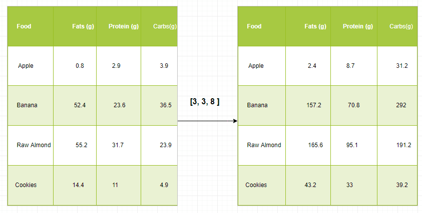
To put it in a more practical context, you often have an array that’s somewhat larger and another one that’s slightly smaller. Ideally, you want to use the smaller array multiple times to perform an operation (such as a sum, multiplication, etc.) on the larger array.
To do this, you use the broadcasting mechanism.
However, there are some rules if you want to use it. And, before you already sigh, you’ll see that these “rules” are very simple and kind of straightforward!
- First off, to make sure that the broadcasting is successful, the dimensions of your arrays need to be compatible. Two dimensions are compatible when they are equal. Consider the following example:
# Import the NumPy library and give it an alias of `np`
import numpy as np

# Initialize a 3x4 array of ones and assign it to the variable `x`
x = np.ones((3,4))

# Print the shape of the array `x`
print("Shape of x:", x.shape)

# Initialize a 3x4 array of random numbers between 0 and 1 and assign it to the variable `y`
y = np.random.random((3,4))

# Print the shape of the array `y`
print("Shape of y:", y.shape)

# Add the arrays `x` and `y` element-wise and print the resulting array
z = x + y
print("Result of x + y:\n", z)

# Print the shape of the resulting array
print("Shape of x + y:", z.shape)- Two dimensions are also compatible when one of them is 1:
# Import the NumPy library and give it an alias of `np`
import numpy as np

# Initialize a 3x4 array of ones and assign it to the variable `x`
x = np.ones((3,4))

# Print the shape of the array `x`
print("Shape of x:", x.shape)

# Initialize a 3x4 array of random numbers between 0 and 1 and assign it to the variable `y`
y = np.random.random((3,4))

# Print the shape of the array `y`
print("Shape of y:", y.shape)

# Add the arrays `x` and `y` element-wise and print the resulting array
z = x + y
print("Result of x + y:\n", z)

# Print the shape of the resulting array
print("Shape of x + y:", z.shape)
Note that if the dimensions are not compatible, you will get a ValueError.
Tip: also test what the size of the resulting array is after you have done the computations! You’ll see that the size is actually the maximum size along each dimension of the input arrays.
In other words, you see that the result of x-y gives an array with shape (3,4): y had a shape of (4,) and x had a shape of (3,4). The maximum size along each dimension of x and y is taken to make up the shape of the new, resulting array.
- Lastly, the arrays can only be broadcast together if they are compatible in all dimensions. Consider the following example:
# Import `numpy` as `np`
import numpy as np

# Initialize `x` and `y`
x = np.ones((3,4))
y = np.random.random((5,1,4))

# Add `x` and `y`
z = x + y
You see that, even though x and y seem to have somewhat different dimensions, the two can be added together.
That is because they are compatible in all dimensions:
- Array x has dimensions 3 X 4,
- Array y has dimensions 5 X 1 X 4
Since you have seen above that dimensions are also compatible if one of them is equal to 1, you see that these two arrays are indeed a good candidate for broadcasting!
What you will notice is that in the dimension where y has size 1, and the other array has a size greater than 1 (that is, 3), the first array behaves as if it were copied along that dimension.
Note that the shape of the resulting array will again be the maximum size along each dimension of x and y: the dimension of the result will be (5,3,4)
In short, if you want to make use of broadcasting, you will rely a lot on the shape and dimensions of the arrays with which you’re working.
But what if the dimensions are not compatible?
What if they are not equal or if one of them is not equal to 1?
You’ll have to fix this by manipulating your array! You’ll see how to do this in one of the next sections.
How do Array Mathematics Work?
You’ve seen that broadcasting is handy when you’re doing arithmetic operations. In this section, you’ll discover some of the functions that you can use to do mathematics with arrays.
As such, it probably won’t surprise you that you can just use +, -, *, / or % to add, subtract, multiply, divide or calculate the remainder of two (or more) arrays. However, a big part of why NumPy is so handy, is because it also has functions to do this. The equivalent functions of the operations that you have seen just now are, respectively, np.add(), np.subtract(), np.multiply(), np.divide() and np.remainder().
You can also easily do exponentiation and taking the square root of your arrays with np.exp() and np.sqrt(), or calculate the sines or cosines of your array with np.sin() and np.cos(). Lastly, its’ also useful to mention that there’s also a way for you to calculate the natural logarithm with np.log() or calculate the dot product by applying the dot() to your array.
Try it all out in the code below.
Just a tip: make sure to check out first the arrays that have been loaded for this exercise!
# Import `numpy` as `np`
import numpy as np
x = np.array([[1, 2, 3], [3, 4, 5]])
y = np.array([6,7,8])

# Add `x` and `y`
z = np.add(x,y)
print("Addition of x and y:\n", z)

# Subtract `x` and `y`
z = np.subtract(x,y)
print("Subtraction of y from x:\n", z)

# Multiply `x` and `y`
z = np.multiply(x,y)
print("Element-wise multiplication of x and y:\n", z)
Remember how broadcasting works? Check out the dimensions and the shapes of both x and y in your IPython shell. Are the rules of broadcasting respected?
But there is more.
Check out this small list of aggregate functions:
| a.sum() | Array-wise sum |
| a.min() | Array-wise minimum value |
| b.max(axis=0) | Maximum value of an array row |
| b.cumsum(axis=1) | Cumulative sum of the elements |
| a.mean() | Mean |
| b.median() | Median |
| a.corrcoef() | Correlation coefficient |
| np.std(b) | Standard deviation |
Besides all of these functions, you might also find it useful to know that there are mechanisms that allow you to compare array elements. For example, if you want to check whether the elements of two arrays are the same, you might use the == operator. To check whether the array elements are smaller or bigger, you use the < or > operators.
This all seems quite straightforward, yes?
However, you can also compare entire arrays with each other! In this case, you use the np.array_equal() function. Just pass in the two arrays that you want to compare with each other, and you’re done.
Note that, besides comparing, you can also perform logical operations on your arrays. You can start with np.logical_or(), np.logical_not() and np.logical_and(). This basically works like your typical OR, NOT and AND logical operations;
In the simplest example, you use OR to see whether your elements are the same (for example, 1), or if one of the two array elements is 1. If both of them are 0, you’ll return FALSE. You would use AND to see whether your second element is also 1 and NOT to see if the second element differs from 1.
Test this out in the code chunk below:
# Import `numpy` as `np`
import numpy as np
# Initialize arrays
a = np.array([1, 1, 0, 0], dtype=bool)
b = np.array([1, 0, 1, 0], dtype=bool)

# `a` AND `b`
np.logical_and(a, b)

# `a` OR `b`
np.logical_or(a, b)

# `a` NOT `b`
np.logical_not(a,b)
How to Subset, Slice, and Index Arrays
Besides mathematical operations, you might also consider taking just a part of the original array (or the resulting array) or just some array elements to use in further analysis or other operations. In such case, you will need to subset, slice and/or index your arrays.
These operations are very similar to when you perform them on Python lists. If you want to check out the similarities for yourself, or if you want a more elaborate explanation, you might consider checking out DataCamp’s Python list tutorial.
If you have no clue at all on how these operations work, it suffices for now to know these two basic things:
- You use square brackets [] as the index operator, and
- Generally, you pass integers to these square brackets, but you can also put a colon : or a combination of the colon with integers in it to designate the elements/rows/columns you want to select.
Subsetting
Besides from these two points, the easiest way to see how this all fits together is by looking at some examples of subsetting:
import numpy as np

# Initialize 1D array
my_array = np.array([1,2,3,4])

# Print subsets
print(my_array[1])
import numpy as np
# Initialize 2D array
my_2d_array = np.array([[1,2,3,4], [5,6,7,8]], dtype=np.int64)
# Print subsets
print(my_2d_array[1][2])
print(my_2d_array[1,2])import numpy as np
# Initialize 3D array
my_3d_array = np.array([[[1,2,3,4], [5,6,7,8]], [[1,2,3,4], [9,10,11,12]]], dtype=np.int64)
# Print subset
print(my_3d_array[1,1,2])Slicing
Something a little bit more advanced than subsetting, if you will, is slicing. Here, you consider not just particular values of your arrays, but you go to the level of rows and columns. You’re basically working with “regions” of data instead of pure “locations”.
You can see what is meant with this analogy in these code examples:
import numpy as np

# Initialize 1D array
my_array = np.array([1,2,3,4])

# Print subsets
print(my_array[0:2])
import numpy as np
# Initialize 2D array
my_2d_array = np.array([[1,2,3,4], [5,6,7,8]], dtype=np.int64)
# Print subsets
print(my_2d_array[0:2,1])import numpy as np
# Initialize 3D array
my_3d_array = np.array([[[1,2,3,4], [5,6,7,8]], [[1,2,3,4], [9,10,11,12]]], dtype=np.int64)
# Print subset
print(my_3d_array[1,...])You’ll see that, in essence, the following holds:
a[start:end] # items start through the end (but the end is not included!)
a[start:]    # items start through the rest of the array
a[:end]      # items from the beginning through the end (but the end is not included!)
In the above code, each array is initialized separately, and subsets are printed in separate code blocks. The my_array, my_2d_array, and my_3d_array are the 1D, 2D, and 3D arrays, respectively, and subsets are printed using the indexing notation.
In the first example, we use slicing to select the items at index 0 and 1 of my_array. In the second example, we use slicing to select the items at row 0 and 1, column 1 of my_2d_array. In the third example, we use the ... notation to select all elements along the first and second dimensions, and the second element along the third dimension of my_3d_array.
Indexing
Lastly, there’s also indexing. When it comes to NumPy, there are boolean indexing and advanced or “fancy” indexing.
(In case you’re wondering, this is true NumPy jargon, I didn’t make the last one up!)
First up is boolean indexing. Here, instead of selecting elements, rows or columns based on index number, you select those values from your array that fulfill a certain condition.
Putting this into code can be pretty easy:
import numpy as np
my_array = np.array([1,2,3,4])
my_3d_array = np.array([[[1,2,3,4], [5,6,7,8]], [[1,2,3,4], [9,10,11,12]]], dtype=np.int64)

# Try out a simple example
print(my_array[my_array<2])

# Specify a condition
bigger_than_3 = (my_3d_array >= 3)

# Use the condition to index our 3d array
print(my_3d_array[bigger_than_3])
Note that to specify a condition, you can also make use of the logical operators | (OR) and & (AND). If you would want to rewrite the condition above in such a way (which would be inefficient, but I demonstrate it here for educational purposes :)), you would get bigger_than_3 = (my_3d_array > 3) | (my_3d_array == 3).
With the arrays that have been loaded in, there aren’t too many possibilities, but with arrays that contain, for example, names or capitals, the possibilities could be endless!
When it comes to fancy indexing, what you basically do with it is the following: you pass a list or an array of integers to specify the order of the subset of rows you want to select out of the original array.
Does this sound a little bit abstract to you?
No worries, just try it out in the code chunk below:
import numpy as np
my_array = np.array([1,2,3,4])
my_2d_array = np.array([[1,2,3,4], [5,6,7,8]], dtype=np.int64)
my_3d_array = np.array([[[1,2,3,4], [5,6,7,8]], [[1,2,3,4], [9,10,11,12]]], dtype=np.int64)

# Select elements at (1,0), (0,1), (1,2) and (0,0)
print(my_2d_array[[1, 0, 1, 0],[0, 1, 2, 0]])

# Select a subset of the rows and columns
print(my_2d_array[[1, 0, 1, 0]][:,[0,1,2,0]])
Now, the second statement might seem to make less sense to you at first sight. This is normal. It might make more sense if you break it down: